OT Security Analytics - Finding the ground truth

In this post, we take a look at analyzing Industrial Control System data to detect unauthorized manipulation of relays in a process.

The problem

Industrial Control Systems (ICS) systems are integral parts of power plants, water and wastewater treatment plants, oil and gas pipelines, as well as many other parts of critical infrastructure. A security breach that takes all or part of the system offline can have far reaching impacts, not just to the corporation or organization, but to local communities and potential economic impacts. If a nuclear power plant, an oil pipeline, or a wastewater treatment plant is compromised, there is high risk for negative environmental impact for many years.

We have seen attacks against ICS in the wild (most famously Stuxnet and the attacks against the Ukranian power grid). Unfortunately, ICS systems are notoriously difficult to secure due to an inverted security model, insecure by design protocols, and an incredibly long shelf life. Situational Awareness can be difficult due to a historical divide of cybersecurity talent and resources between Operational Technology and Information Technology (OT vs IT). The Gravwell founders have their roots in this industry and know the problem well.

This case study focuses on a particular ICS process in which a relay is activated without the operator being made aware via the process monitoring display. Losing control of the process is the ultimate worst case scenario for any operator or ICS engineer. Further, forensics to detect the extent of an attack are practically nonexistent -- logs from ICS equipment are very rare, let alone security-specific information, and when they do exist they are vulnerable to being lied to by an attacker.

The Gravwell Solution

Gravwell was built to be flexible about how we ingest and process data. This enables us to go places that most data analytics companies simply cannot. ICS systems often rely on lesser known or proprietary binary protocols. The Gravwell pipeline analytics approach allows for ingestion of any kind of data and then, at process time, intelligence is extracted at a low level and built upon to create actionable intelligence.

With a worldwide shortage of cybersecurity talent, it was important for us to make the job easier for everyone and to maximize the resources an organization does have. Gravwell visualizations and dashboard displays are usable by non-technical personnel and operators. In the event of an anomaly or incident requiring further investigation, the underlying data is always present and an escalation up to a hunt team can go from tip to final solution without leaving Gravwell.

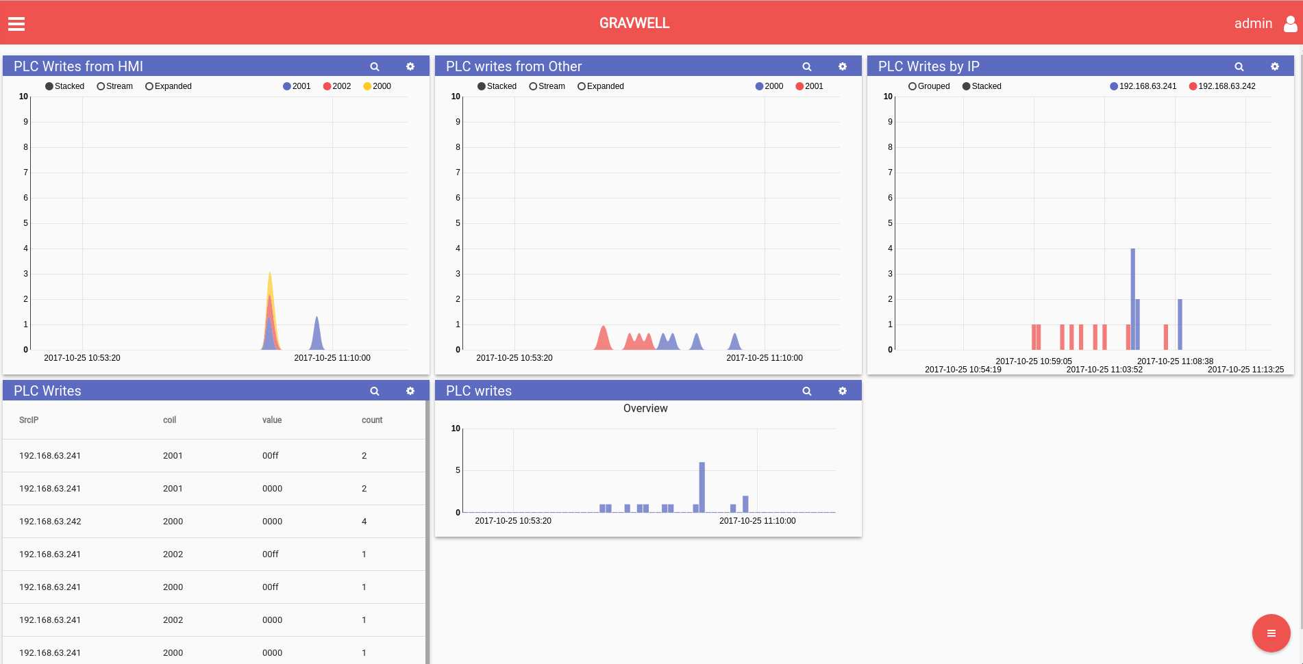
To solve the situational awareness problem and detect any activity altering the process we built out a dashboard to show a breakdown of PLC write requests from the HMI (“authorized”) vs those from alternate sources (“unauthorized”) along with some asset discovery. The authorized activity is in the upper left chart and unauthorized in the upper middle with other charts for monitoring the process. By displaying the information in this way, it becomes trivial to spot and investigate unauthorized attempts to control the PLC.

Details Breakdown

This section covers a technical dive into everything that went into the analytics and discovery for this problem, starting from nothing.

Asset Discovery

For the Gravwell analysis of the system, let's assume we know nothing about it and start off with some asset discovery. We want to find out which systems are present on our network and how they are talking. To get this data, we're feeding Gravwell a pcap of network activity from these hosts in the control system. Alternatively, we could feed Gravwell via a span port and have real-time and historical analysis of our process.

The first query we'll run is a basic chart of network activity:

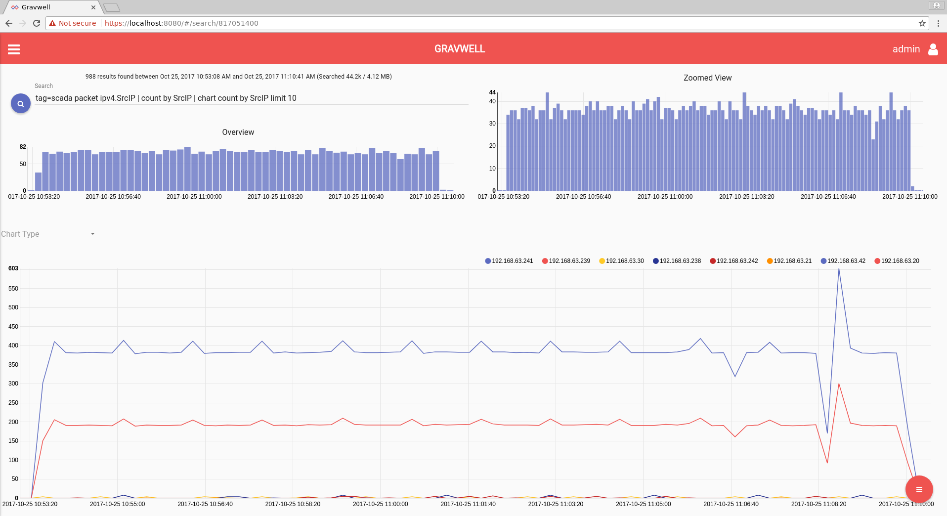
```tag=scada packet ipv4.SrcIP | count by SrcIP | chart count by SrcIP limit 10```

This gives us a quick and easy way to see who our biggest talkers are on this network. Looks like we've got .241 and .239 as our primary communicators.

Let's build out some high level force directed graphs to get a handle on which machines are communicating and how. The following two force directed graphs are built out with similar queries. This first graph shows all servers on the network and the ports on which they communicate (this is a great query you probably want to bookmark).

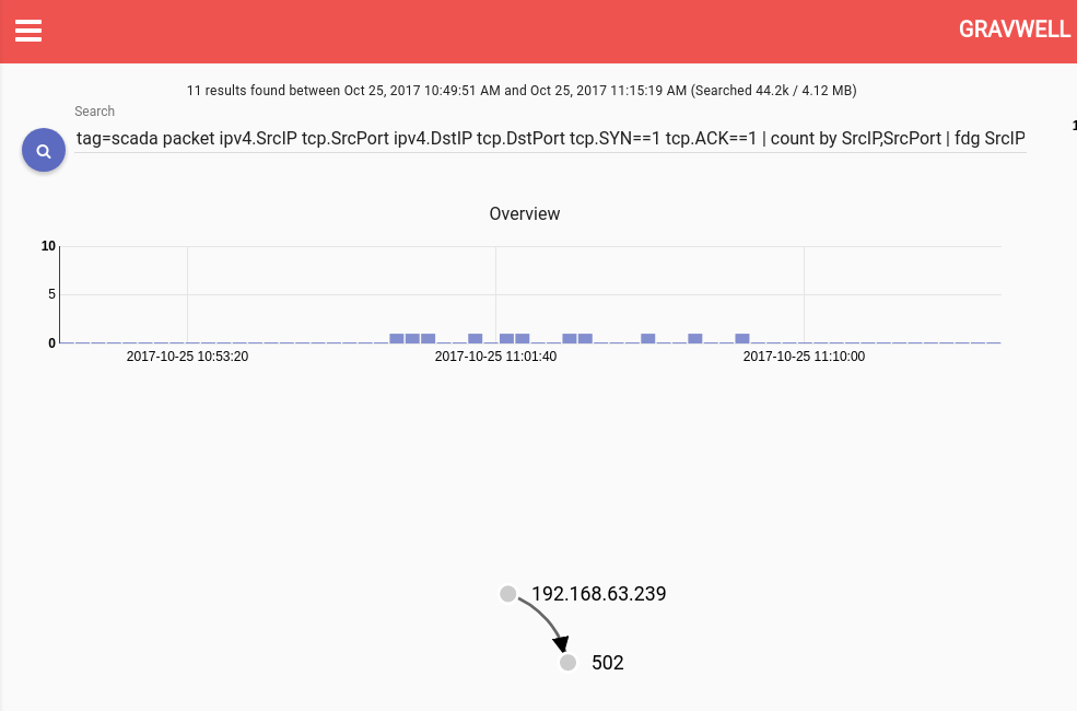
```tag=scada packet ipv4.SrcIP tcp.SrcPort ipv4.DstIP tcp.DstPort tcp.SYN==1 tcp.ACK==1 | count by SrcIP,SrcPort | fdg SrcIP SrcPort```

In this pcap excerpt, we observe a single service running at address .239 on port 502. If you're familiar with SCADA protocols at all, you might recognize that as Modbus over TCP.

Let's build out a graph of server-client connections.

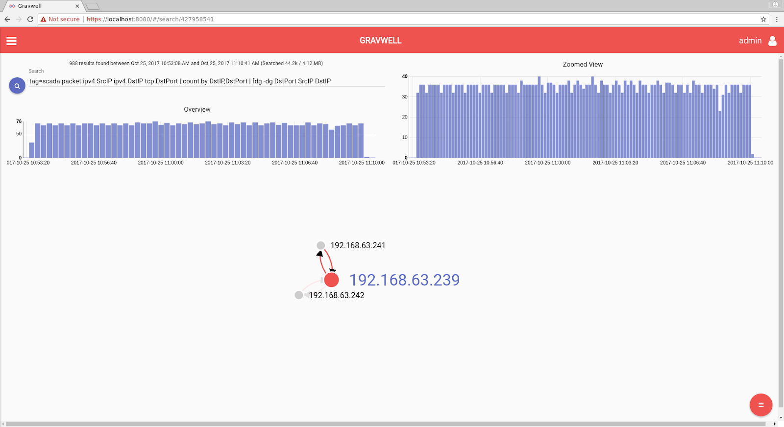
```tag=scada packet ipv4.SrcIP ipv4.DstIP tcp.DstPort | count by DstIP,DstPort | fdg -dg DstPort SrcIP DstIP```

Similar to the previous query, we are using force directed graphs to plot traffic between servers and clients. The darker the lines, the more traffic occurs between these nodes on the graph. We can see that .293 has had two clients connect to it, .241 and .242. This is expected given our earlier analysis.

Network flows give us some rapid insight into what's happening. Now that we've figured out we have some server listening on port 502 and serving to one client at high frequency and another client infrequently, let's dive into analysis of the actual underlying process data.

OT Analytics

It looks like this process is using TCP Modbus for command and control. In summary, this protocol is used to find out if something is on or off and to tell things to turn on or off.

Let's do a brief Modbus primer for those unfamiliar. Feel free to skip ahead if you're less interested in the underlying 1s and 0s.

A Brief Modbus Primer

Modbus is a communications mechanism created in 1979 for controlling PLCs. The Modbus protocol was originally designed for serial links and has gone through some changes over the years -- both in terms of the protocol and in general practical usage. This control system uses Modbus over TCP. For this analysis we're going to be doing some low level bit carving right in the Gravwell search pipeline to demonstrate that 1) Gravwell can get actual ground truth data about your running process and 2) Gravwell can work on ANY data, even proprietary undocumented protocols.

Warning: incoming hex.

Modbus over tcp has a fairly straightforward format. The header officially has 7 bytes (but actually 8 if you include the function code). It includes a 2 byte transaction number, two bytes of protocol (always 0 in our case here), two bytes of payload length, and one byte for the unit ID.

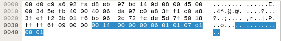
This is an example of a Modbus over TCP packet. In this case, the transaction number is 0x14, the protocol is 0, the length is 6, and the unit is 1. The next byte is the function code, which determines what action the message requires. Let's go through the actions we're going to be seeing.

Status Requests

Requests for the current process status are done via modbus function code 1, which officially is "Read Discrete Output Coils" or in layman's terms, "Is this thing on or off?" The request message includes the "coil" address and the number of coils that are to be read and returned. This is an unused legacy capability as any requests in this control system are for single data points at a time.

Looking at our example request hex again, the remaining message consists of a single byte function code, a two byte "coil address", and a two byte "read length" which allows requests of multiple coils. In this control system the read length is always 1 as requests for different coils are made separately.

With the example hex from above, the function code is 1 and the coil address is 2001.

Here is the response from the PLC:

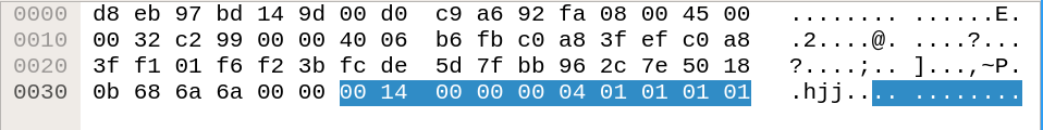
The PLC response is very basic and includes the common header format plus the modbus payload. The 0x1's are the unit ID, function code, length, and finally the actual data. So this message indicates a response that coil 2001 is currently set to 1 or "on". Note that the response does not contain the coil address, it is tied to the request via the transaction ID

Change Requests

Function code 1 is a "read" function code to get current status. Now we'll dive into the "write" function codes that are active in this system. Let's look at an example change request.

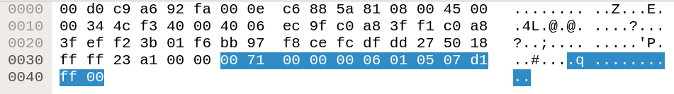
Parsing out the message we see that the function code is 5, the address is 2001, and the data is 0xFF00.

The response from the server is simply an echo of this message.

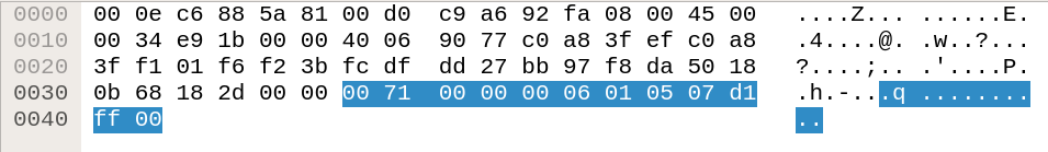
For posterity, let's look at the function 1 responses before and after this message.

Before
After

The last byte changes from a 0 to a 1 as the write message goes through and alters the physical state of the process causing the relay to close.

Gravwell OT Analytics

Now that we've got a baseline understanding about what's happening under the hood in this process, let's get to the actual fun part -- analytics! Gravwell was built to be data agnostic, we can handle data of any kind be it logs, video, or control system protocols. For this analysis we'll use the built-in Gravwell Modbus protocol analysis. We'll leave the final bits of analytics up to Gravwell low-level byte slicing modules to demonstrate that Gravwell can handle ANY kind of protocol, be it a well defined standard or something unique and proprietary (which is not uncommon in Industrial Control Systems).

Gravwell has a Modbus parsing agent built into the packet analyzer. This search shows all extracted Modbus fields:

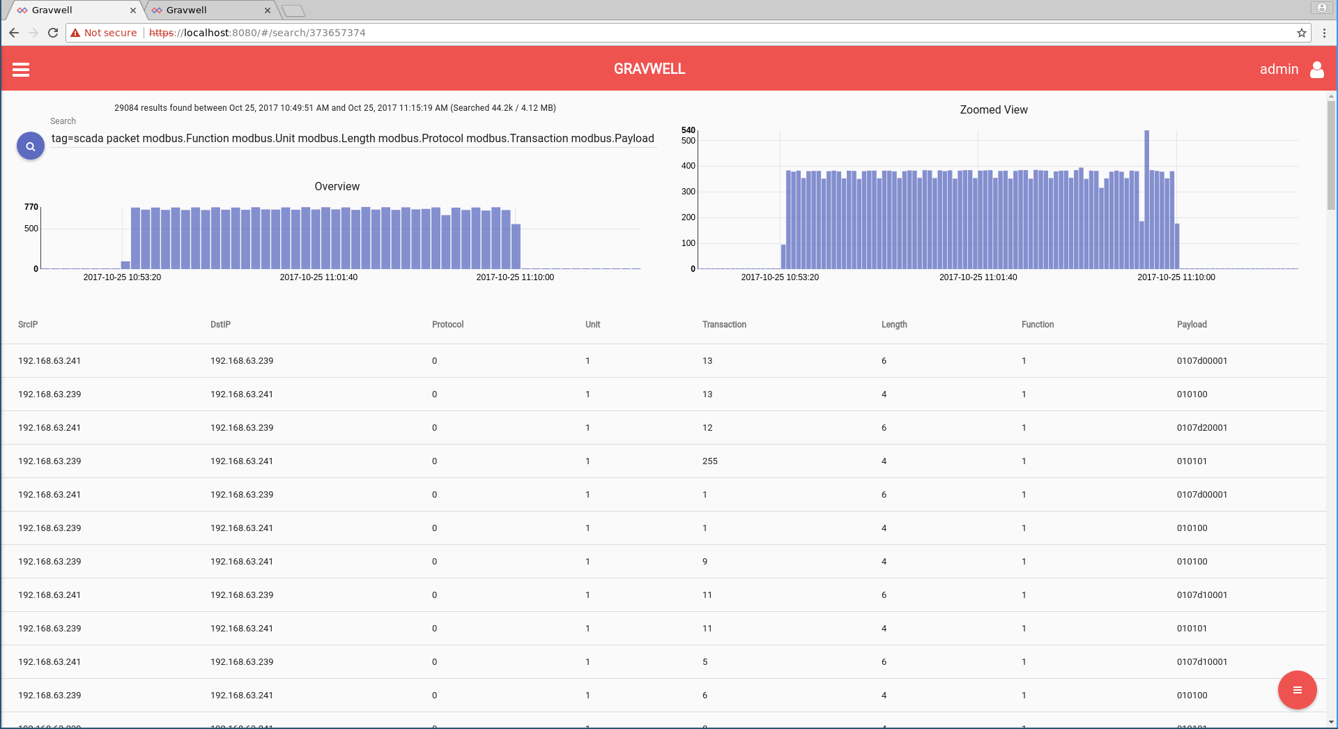
```tag=scada packet modbus.Function modbus.Unit modbus.Length modbus.Protocol modbus.Transaction modbus.Payload ipv4.SrcIP ipv4.DstIP | hexlify Payload | table SrcIP DstIP Protocol Unit Transaction Length Function Payload```

Let's issue an initial search to determine which request function codes are actually in use on the system and who is sending them.

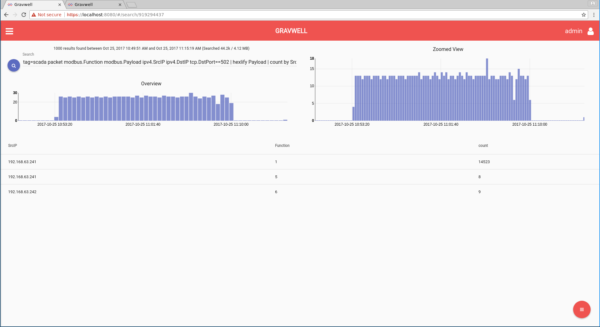
```tag=scada packet modbus.Function modbus.Payload ipv4.SrcIP ipv4.DstIP tcp.DstPort==502 | hexlify Payload | count by SrcIP,Function | table SrcIP Function count```

This query shows us that the only function codes in use are 1, 5, and 6 while also raising some suspicions. We can see .241 reading and occasionally writing to the PLC. The .242 address, however, never issues a read and only writes to the PLC with function code 6.

Let's get to the bottom of this and search for all IPs writing to the PLC.

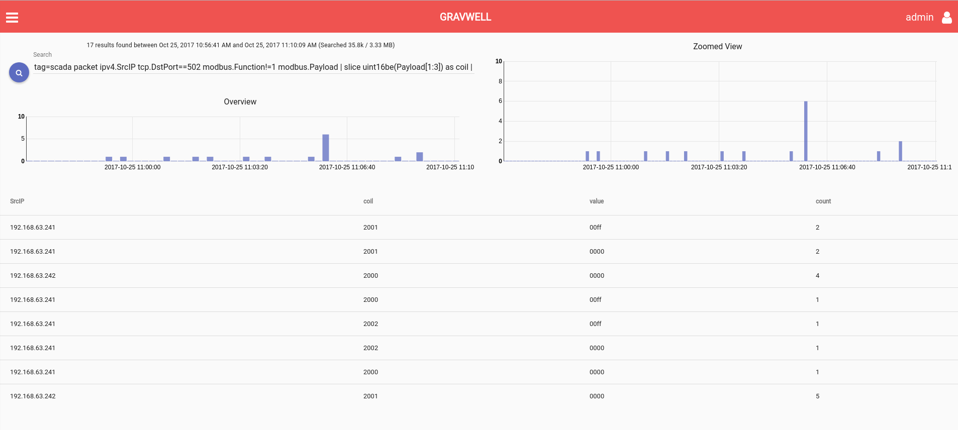
```tag=scada packet ipv4.SrcIP tcp.DstPort==502 modbus.Function!=1 modbus.Payload | slice uint16be(Payload[1:3]) as coil | slice uint16be(Payload[3:5]) as value | hexlify value | count by SrcIP,coil,value | table SrcIP coil value count```

Looking at this chart it's clear to see that .242 is either a misconfigured system or an attacker controlling the process. This kind of attack is often impossible to see from the process HMI itself, unfortunately, due to limitations in the protocol and equipment. Extra analytics of the kind that Gravwell provides are required.

Finally, let's take these queries and build out a dashboard that gives us full insight into what is communicating with these ICS components and increase our situational awareness on who, when, and how changes are being written to the PLC.

This dashboard provides a holistic view into everything that's interacting with our PLC. In this case, we're only looking at a single PLC in a process. Altering the queries to monitor multiple PLCs is straightforward.

For a final point, let's run a basic search and discover the ethernet MAC address belonging to this system so we can lookup the specific switch and port in order to find the physical machine.

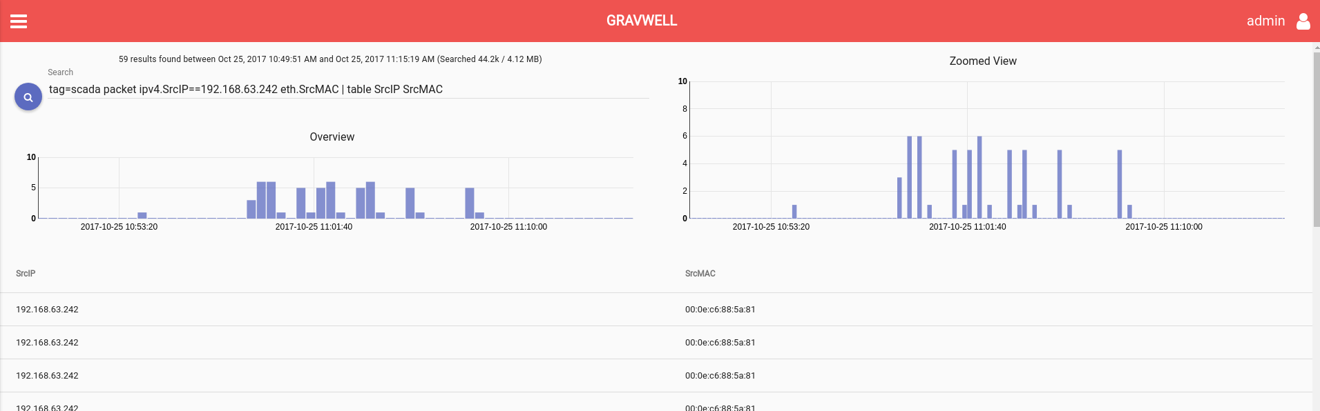
Gotcha! Thanks Gravwell.

Final Thoughts

This case study has walked through specifics for monitoring a PLC driving some power relays. We started with asset discovery, built some specific queries for monitoring, and finally created a dashboard for easy viewing if we want to revisit this type of information in the future. Using the situational awareness gained from the data, we discovered a rogue or misconfigured system interacting with our process and are prepared to hunt the specific switch and port to which the MAC address belongs.

The power of Gravwell lies in its flexibility, both in it's capability and applicability. Gravwell can hunt data of any kind in any environment and it's built to help your team do more. Gravwell can be utilized by savvy cyber ninjas and operational technicians alike.

Try Gravwell

With Gravwell Community Edition, you are able to unlock the power of Gravwell at your place of work or in your Homelab. A license is free and allows you to ingest up to 13.9 GB a day of ingestion. Request a license by clicking on the button below.

Once you are up and running, stop by our Discord and share comments or ask questions with the Gravwell Dev Team: