We've had some benchmarking requests from multiple organizations struggling with ingest performance from Elasticsearch, so we're publishing them here. The latest Gravwell release marks a significant improvement in ingest and indexing performance and this post covers the nitty gritty details. Better ingest performance means reduced infrastructure cost, less dropped data, and faster time-to-value. See how Gravwell stacks up.
When doing some comparisons of Gravwell to other systems, it's important to remember that Gravwell is an unstructured system -- more of a data lake than a data warehouse. So while some competitors convert the data into a fully structured document for ingest and indexing, Gravwell does this all on the fly with a highly flexible data definition. So even if a log entry contains a stack trace (we have seen that... a lot) Gravwell can still ingest it and you can still query it. Anomalous input does not break core Gravwell indexing. We'll talk more about that distinction in a future post, but for now let's jump right into the results.
The core results from the Elasticsearch benchmark are generated from a 3.2GB geoname dataset in JSON format using the esrally tool. This is structured data. To better serve our customers unique needs, Gravwell has a modular indexing strategy. The worst case "shotgun" approach is to just full text everything.
Elasticsearch and Gravwell are very different systems at their core and each solves different problems. Apples-to-apples comparisons aren't really fair, so keep that in mind. However, many people use Elasticsearch for log and event correlation and analytics so....here we go:
| Platform | Ingest Rate | Ingest Size on Disk |
| Elasticsearch (best case) | 65K EPS | 3.5X |
| Gravwell (worst case) | 65K EPS | 1.6X |
| Gravwell (best case) | 530K EPS | 1.12X |
Keep reading for the technical details or skip to raw output at this gist.
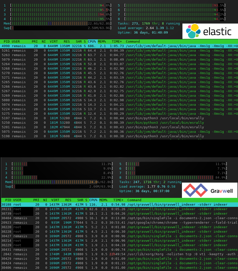
The other thing to point out is the system utilization during ingest. Here are two screenshots of htop running during these benchmarks.
The Gravwell paradigm of "ingest anything" means standing up Gravwell can be insanely fast and easy compared to complicated structure-on-ingest solutions. Get your log analytics set up in hours instead of days.

Test System
For this blog we will be leveraging an Intel Core i7-7700k. This system is not a server class system with quad, hexa, or even octo channel memory, but it has characteristics similar to what you might find in a low cost 1U blade server. We will also be running our instance of Gravwell inside Docker and using the BTRFS filesystem.
The exact specs are:
| Component | Details |
| Intel Core i7-7700k | 4.2Ghz base and 4.5Ghz Boost clock 86MB of cache |
| 32GB DDR4-2400 | Crucial 2400Mhz DDR4 across 2 DIMMS |
| 960GB NVME SSD | Samsung 960 EVO |
| Linux Kernel 4.15.0 | Ubuntu Bionic 4.15.0-47-generic |
| Docker 18.09.2 | Git commit 6247962 |
We will show a variety of configurations with different indexing schemes and engines so that you can see how the various configurations effect ingest and query performance.
System Tuning
Not much tuning is needed with a modern Linux system with Gravwell, but a few tweaks can reduce the strain and wear and tear on hardware components when using the index engine. Mostly we are trying to reduce the number of page writebacks that occur when the host system has a very fast disk available. Gravwell uses a synchronization system to ensure that data makes it to the disk, but the host kernel will also attempt to push dirty pages back to the disk as it can. Fast disks, like NVME flash, allow the kernel to perform these writebacks very quickly which can cause needless flash wear and tear. If you do not tune these parameters your performance won't change much, but you might see a lot more data written to your SSD.
Four parameters in the virtual memory subsystem should be tweaked:
- dirty_ratio
- dirty_background_ratio
- dirty_writeback_centisecs
- dirty_expire_centisecs
Here is a handy script that will throw some good values in and set them up to be reloaded at every reboot.
#!/bin/bash
user=$(whoami)
if [ "$user" != "root" ]; then
    echo "must run as root"
fi

echo 70 > /proc/sys/vm/dirty_ratio
echo 60 > /proc/sys/vm/dirty_background_ratio
echo 2000 > /proc/sys/vm/dirty_writeback_centisecs
echo 3000 > /proc/sys/vm/dirty_expire_centisecs

echo "vm.dirty_ratio = 70" >> /etc/sysctl.conf
echo "vm.dirty_background_ratio = 60" >> /etc/sysctl.conf
echo "vm.dirty_writeback_centisecs = 2000" >> /etc/sysctl.conf
echo "vm.dirty_expire_centisecs = 3000" >> /etc/sysctl.conf
Methodology
We will be using Gravwell version 3.1.0 and ingesting text data using the singleFIle ingester from gravwell ingesters on commit e6c6fadfdf507e9bffc5e3cb930b9d07ca5c0719. Ingest will be performed with the "-ignore-ts" flag so that ingest rates are not limited by the single ingesters ability to resolve timestamps dynamically.
For each configuration we will flush the file system caches on the host prior to ingest and query using the command:
sync; echo 3 > /proc/sys/vm/drop_caches
The docker system is mounted on its own partition using the BTRFS filesystem with transparent file compression. When we use the transparent file compression we will use the ZSTD compression algorithm with compress-force=true. The exact /etc/fstab entry for storage volume is:
/dev/nvme0n1p4 /var/lib/docker btrfs ssd,compress-force=zstd 0 0
Well Configurations
Each data set will be ingested using four different well configurations:
- No indexing at all, only a temporal index
- Fulltext indexing, worst case
- Complete field indexing using the bloom engine
- Complete field indexing using the index engine
Raw Well
This well utilizes no data indexing at all, just a raw unstructured ingest. The well DOES build a temporal index, but because the data does not have timestamps the temporal index is minimal. Every query will need to scrape and structure the entire dataset.
[Storage-Well "raw"]
    Location=/opt/gravwell/storage/raw
    Tags=raw
    Enable-Transparent-Compression=true
Fulltext Well
This well utilizes the fulltext accelerator and will break every log entry into its components for indexing using the index engine. This is by far the most abusive indexing strategy, but is also the most forgiving. Fulltext indexing allows you accelerate searches on subcomponents, not just complete fields. The fulltext indexing system can often result in an index that is as large or larger than the original data.
[Storage-Well "fulltext"]
    Location=/opt/gravwell/storage/fulltext
    Tags=fulltext
    Accelerator-Name=fulltext
    Accelerator-Engine-Override=index
    Enable-Transparent-Compression=true
Field Extraction With Bloom Engine Well
The field extraction system extracts each field and uses Gravwell's bloom engine to perform query acceleration. The bloom engine is much more efficient when comes to disk overhead, but can be less efficient for query. Bloom filters provide the ability to say that a field value is definitely not in a set, or might be in a set. Gravwell uses the bloom engine to rapidly evaluate whether or not it needs to process a block of data, effectively reducing the search space. The bloom engine performs very well when querying sparse data, but is not very effective when querying fields that occur regularly.
[Storage-Well "bench"]
    Location=/opt/gravwell/storage/bench
    Tags=bench
    Accelerator-Name=<dataset dependent>
    Accelerator-Args=<dataset dependent>
    Accelerator-Engine-Override=bloom
    Enable-Transparent-Compression=true
Field Extraction With Index Engine Well
Field extraction with the indexing system uses a full indexing solution combined with field extraction. The indexing engine can consume significant disk space (especially if paired with full text indexing), but provides an effective acceleration across all query types, sparse and dense. However, that disk overhead can translate to dramatic query speedups, especially when dealing with extremely large data sets.
[Storage-Well "bench2"]
    Location=/opt/gravwell/storage/bench2
    Tags=bench2
    Accelerator-Name=<dataset dependent>
    Accelerator-Args=<dataset dependent>
    Accelerator-Engine-Override=index
    Enable-Transparent-Compression=true
Installing gravwell.conf and Starting
To start, make sure that you have the latest Gravwell docker image by performing a docker pull gravwell/gravwell:latest, then create the container without starting it:
docker create --name benchmark --rm gravwell/gravwell:latest
Pull the default gravwell.conf from the container, edit it to add our wells (there will be 8 plus the default), push it back in, and then start the container:
docker cp benchmark:/opt/gravwell/etc/gravwell.conf /tmp/
vim /tmp/gravwell.conf
docker cp /tmp/gravwell.conf benchmark:/opt/gravwell/etc/gravwell.conf
docker start benchmark
The exact gravwell.conf we will be using is:
[global]
### Web server HTTP/HTTPS settings
Web-Port=80
Insecure-Disable-HTTPS=true

### Other web server settings
Remote-Indexers=net:127.0.0.1:9404
Persist-Web-Logins=True
Session-Timeout-Minutes=1440
Login-Fail-Lock-Count=4
Login-Fail-Lock-Duration=5

[Default-Well]
    Location=/opt/gravwell/storage/default/
    Disable-Compression=true

[Storage-Well "rawgeo"]
    Location=/opt/gravwell/storage/rawgeo
    Tags=rawgeo
    Enable-Transparent-Compression=true

[Storage-Well "fulltextgeo"]
    Location=/opt/gravwell/storage/fulltext
    Tags=fulltextgeo
    Accelerator-Name=fulltext
    Accelerator-Engine-Override=index
    Enable-Transparent-Compression=true

[Storage-Well "benchgeo"]
    Location=/opt/gravwell/storage/benchgeo
    Tags=benchgeo
    Accelerator-Name=fields
    Accelerator-Args="-d \"\t\" [0] [2] [3] [4] [5] [6] [7] [8] [9] [10] [11] [12] [13] [14] [15] [16] [17]"
    Accelerator-Engine-Override=bloom
    Enable-Transparent-Compression=true

[Storage-Well "bench2geo"]
    Location=/opt/gravwell/storage/bench2geo
    Tags=bench2geo
    Accelerator-Name=fields
    Accelerator-Args="-d \"\t\" [0] [2] [3] [4] [5] [6] [7] [8] [9] [10] [11] [12] [13] [14] [15] [16] [17]"
    Accelerator-Engine-Override=index
    Enable-Transparent-Compression=true

[Storage-Well "rawapache"]
    Location=/opt/gravwell/storage/rawapache
    Tags=rawapache
    Enable-Transparent-Compression=true

[Storage-Well "fulltextapache"]
    Location=/opt/gravwell/storage/fulltextapache
    Tags=fulltextapache
    Accelerator-Name=fulltext
    Accelerator-Engine-Override=index
    Enable-Transparent-Compression=true

[Storage-Well "benchapache"]
    Location=/opt/gravwell/storage/benchapache
    Tags=benchapache
    Accelerator-Name=fields
    Accelerator-Args="-q -d \" \" [0] [1] [2] [3] [5] [6] [7] [8] [9] [10]"
    Accelerator-Engine-Override=bloom
    Enable-Transparent-Compression=true

[Storage-Well "bench2apache"]
    Location=/opt/gravwell/storage/bench2apache
    Tags=bench2apache
    Accelerator-Name=fields
    Accelerator-Args="-q -d \" \" [0] [1] [2] [3] [5] [6] [7] [8] [9] [10]"
    Accelerator-Engine-Override=index
    Enable-Transparent-Compression=true
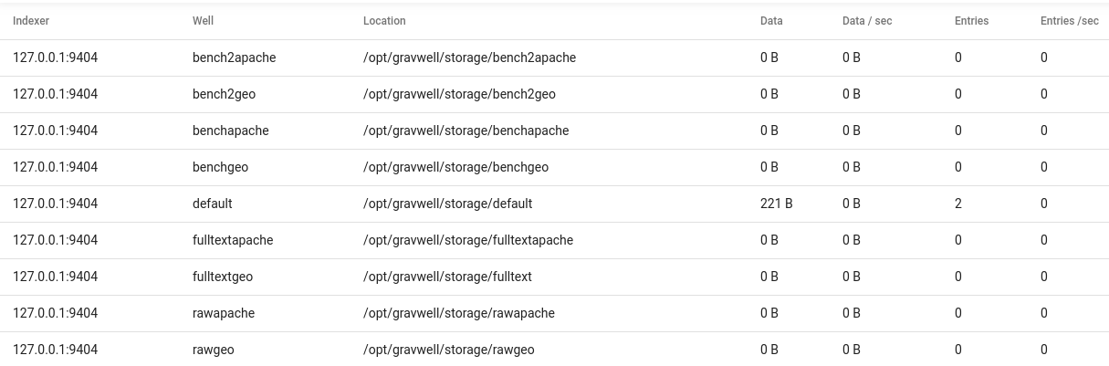
The docker image has the ingest and control secrets configured via environment variables, so we do not need to set them in the gravwell.conf. We can now upload our license and check on our well configurations through the GUI.
Data Sets and Results
For familiarity, we will be using some of the same datasets employed by Elastic.co to benchmark elasticsearch. The datasets are all available on github and represent a nice cross section of data types that might be stored in Gravwell. Here are links to benchmarking info on Elasticsearch and Lucene itself.
Some of the data sets have very high key variability (many completely unique fields) and some have relatively low key variability (reasonable amount of key repetition). In most networking and security contexts key variability is relatively modest as the same machines will typically do the same things over and over.
The command used to ingest each data set using the singleFile ingester is roughly:
Installing the singleFile ingester is as simple as running "go get -u github.com/gravwell/ingesters/singleFIle" if you have the go tools installed.
Geonames
The geonames data set contains a tab delimited data set of locations around the world. The fields include unique identifiers, country codes, city names, locations, elevations, coordinates, etc. This dataset has a very high level of key variability. Every single entry contains multiple unique values, including IDs, coordinates, locations, elevations, and populations. The geonames data set is a good example of ingesting data that is particularly abusive to an index.
The geonames dataset is comprised of 11.9 million records and 1.5GB. The raw data is available at via geonames.org and is described on their readme page. Gravwell will use the fields acceleration module to handle the tab delimited data for the bench and bench2 wells.
The Accelerator-Name parameter will be fields and the Accelerator-Args parameter will use the tab delimiter and will index the full 18 fields.
Accelerator-Name=fields
Accelerator-Args="-d \"\t\" [0] [1] [2] [3] [4] [5] [6] [7] [8] [9] [10] [11] [12] [13] [14] [15] [16] [17]"
| Well | EPS KE/s | Ingest Rate MB/s | Disk Usage | Uncompressed Size |
| Raw | 586.11 | 71.28 | 437 MB | 1.8 GB |
| Fields Bloom | 494.30 | 60.11 | 573 MB | 1.9 GB |
| Fields Index | 98.07 | 11.93 | 2.1 GB | 3.5 GB |
| Fulltext | 76.21 | 9.27 | 2.1 GB | 3.5 GB |
| The median rate of ingestion for Elastic | 65K EPS |
| The size on disk for Elastic | 3.5X original size (5.8GB Index, 2.7GB Translog, 3GB Store, 17GB total written) |
| The mean rate of ingestion for Fulltext indexing Gravwell (the worst case scenario for Gravwell) | 65K EPS |
| Size on disk for Fulltext Indexing Gravwell | 1.6X original size (1.6G index, 3.7GB Store) |
| The mean rate of ingestion for JSON structured indexing for Gravwell | 100K EPS (1.6X size on disk) |
| The mean rate of ingestion for Bloom Filtered JSON indexing for Gravwell | 388K EPS (1.15X size on disk) |
| The mean rate of ingestion for Time Series Only indexing for Gravwell | 530K EPS (1.12X size on disk) |
Apache Access Logs
A common log format used to benchmark indexing systems is the Apache access log. There aren't very many large corpus of access logs available, so we used a generator from github to generate 10 million apache access logs that take up 2.1 GB of space. The generator used to generate the log data is available Fake Apache Log Generator.
The Accelerator-Name parameter will be fields and the Accelerator-Args parameter will use the space delimiter and supported quoted fields, we will index the full 9 fields.
Accelerator-Name=fields
Accelerator-Args="-q -d \" \" [0] [1] [2] [3] [4] [5] [6] [7] [8] [9]"
| Well | EPS KE/s | Ingest Rage MB/s | Disk Usage | Uncompressed Size |
| Raw | 538.28 | 113.16 | 531 MB | 2.4 GB |
| Fields Bloom | 446.35 | 93.87 | 605 MB | 2.2 GB |
| Fields Index | 123.89 | 26.06 | 1.6 GB | 3.5 GB |
| Fulltext | 94.26 | 19.82 | 904 MB | 3.4 GB |
Interestingly, the uncompressed storage usage on indexing the whole fields uses more disk space than just indexing the entire entry with fulltext. There are a pretty standard set of useragent components and URL components and when you combine them they become pretty unique keys. When you treat them as words, there isn't much variability so fulltext is actually a bit more efficient in terms of disk space here.
Query Performance
To measure query performance we will run two queries across each well, the first query finds the raw record using a sparse data field (we will use an IP or city name), the second query uses a dense field (we will use a request and country code). Thow two queries will show the performance characteristics of each indexing method. For each query result we will provide the total time to execute as well as the total number of entries that enter the search pipeline. Examining the total number of entries that enter the pipeline is a good metric for determining how effective the indexing system was at reducing the search space.
GeoNames
For the GeoName data set we will execute two queries for each well, the first is a query that retrieves a single record using a highly unique key, the second is one that retrieves some subset of the records using a reasonably common key. We will use the fields module with inline filtering for all wells except the fulltext well where we will use the grep module and the "-w" flag.
Sparse Query Results
For this test we will retrieve a single record using a unique identifier, we will be pulling back the geonames entry for the Moscow, ID police department with the unique ID 9671688.
The exact query for the fields wells is:
fields -d "\t" [0]==9671688
The query for the fulltext well is:
grep -w 9671688
| Well | Query Time | Entries Entering Pipeline | Query Efficiency |
| Raw | 3.22 s | 11,902,271 | ~ 0 % |
| Fields Bloom | 271.5 ms | 23,321 | 99.8 % |
| Fields Index | 124.9 ms | 1 | 100 % |
| Fulltext | 130.9 ms | 1 | 100 % |
Dense Query Results
For this test we will retrieve a subset of records using a relatively common identifier, we will be pulling every item in the "America/Boise" region. Because the field contains a word separator or fulltext query will have to filter terms. There are 25,263 entries out of the 11.9 million that match this query.
The exact query for the fields wells is:
fields -d "\t" [17]=="America/Boise"
The query for the fulltext well is:
grep -w -s America Boise | grep "America/Boise"
| Well | Query Time | Entries Entering Pipeline | Query Efficiency |
| Raw | 4.69 s | 11,902,271 | ~ 0 % |
| Fields Bloom | 517.6 ms | 761,100 | 94 % |
| Fields Index | 290.2 ms | 25,263 | 100 % |
| Fulltext | 568.2 ms | 25,263 | 100 % |
Apache Access
For the Apache access log data set we will again execute two queries for each well, the first is a query that retrieves a single record filtering for a specific IP, the second is one that retrieves some subset of the records using a reasonably common key. We will use the fields module with inline filtering for all wells except the fulltext well where we will use the grep module and the "-w" flag.
For this test we will retrieve a single record by searching for a specific IP; for the well using fulltext well we will use "grep -w" to find a specific record, for all others we will use the fields module to extract a specific field.
Sparse Query Results
For the sparse search, we are going to look for logs from a specific IP. Because we used a generator and have less than 4 billion records, there is a reasonable likelihood that each IP is only in the log set once or twice. We are looking for the IP 104.170.11.4, but if you are following along you will need to pick an IP in your set.
The exact query for the fields wells is:
fields -d " " -q [0]=="104.170.11.4"
The query for the fulltext well is:
grep -w "104.170.11.4"
| Well | Query Time | Entries Entering Pipeline | Query Efficiency |
| Raw | 3.42 s | 10,000,000 | ~ 0 % |
| Fields Bloom | 253.5 ms | 16,530 | 99.8 % |
| Fields Index | 147.8 ms | 1 | 100 % |
| Fulltext | 143.5 ms | 1 | 100 % |
Dense Query Results
For the dense query search, we are going to look for entries with a return code of 500. The 500 error code represents about 2% of the log entries in our data set. Because the "word" 500 might be in other places, the "grep -w" module can't stand on its own, so we have to follow it up with another grep to ensure we are only getting entries with a return code of 500.
The exact query for the fields wells is:
fields -d " " -q [6]==500 | count
The query for the fulltext well is:
grep -w 500 | grep " HTTP/1.0\" 500"
| Well | Query Time | Entries Entering Pipeline | Query Efficiency |
| Raw | 3.46 s | 10,000,000 | ~ 0 % |
| Fields Bloom | 3.34 s | 10,000,000 | ~ 0 % |
| Fields Index | 2.88 s | 200,102 | 100 % |
| Fulltext | 3.15 s | 200,102 | 100 % |
It is important to note how the bloom engine utterly failed for this dense query, this is because the bloom engine can only say if some is or is not in a set. For this query and data set, the return code of 500 was evenly spread throughout the entire dataset; it was likely in every single block, making the bloom engine acceleration not much better than raw. It is important to think about your queries and your data. The bloom engine is great for finding needles in a haystack, but pretty terrible at dealing with subsets that are relatively dense.
The results for these queries are a lot less spectacular than the sparse queries due to the even disbursement of our target dataset. Most of the work is done pulling data from the disk and decompressing blocks, so while the index engine ensured that very few entries entered the pipeline, the storage system still had to do a lot of work to get blocks off the disk.
Conclusion
Gravwell provides significant flexibility in how and what it indexes. Logging and data analytics systems are typically sized for a median data flow, whether that be EPS or MB/s, however the real world often throws wrenches and it can be extremely important to have the ingest and indexing headroom to deal with sudden bursts of data.
The hybrid indexing system also enables users of the system to not need to know exactly how data is indexed; as long as they leverage inline filters and the appropriate filtering modules Gravwell will use the configured accelerators to speed up queries. Queries that span multiple tags and wells will transparently invoke their respective acceleration engines without user involvement.