The Gravwell team is happy to announce the release of Gravwell 4.1.0 - Gamma Burst.
A few highlights of what's included in the new release:
- Compound Query support
- Web UI based ingester
- A new “enrich” module
- Temporal mode in the “dump” module
- Internal performance and stability improvements
(Current users - visit the download page for instructions on updating. For a complete list of changes, see the Gravwell 4.1.0 release notes)
We’ll have a series of blog posts discussing the various features of Gravwell 4.1.0, but we wanted to get started with our favorites - Compound Queries.
Compound Queries
Collecting data from various data sources, normalizing that data across multiple formats, and then attempting to enrich or correlate otherwise unrelated datasets in a single query is the living nightmare of many cybersecurity professionals.
Thankfully, Gravwell has put their top people on exactly this problem, and the result is a new feature in Gravwell 4.1.0 - Compound Queries. 🎉 Compound Queries is an addition to the query language that allows you to perform multiple, in-order, queries, and use the output from a previous query anywhere in the pipeline of the next, similar to an SQL JOIN.
In other words, Compound Queries allows you to take data from multiple (in fact, any number of) datasets and combine them in in various ways.
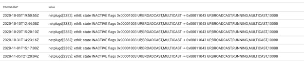
Let’s look at an example from my home - my internet service regularly goes down. I see this activity from the syslog output from my border router with a simple query:
tag=syslog ax value~”eth0: state INACTIVE”
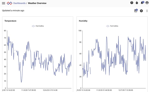
I’ve long since suspected that the weather, specifically the humidity, has something to do with these interruptions, and luckily I have a great weather dataset already in Gravwell thanks to the Weather Kit!
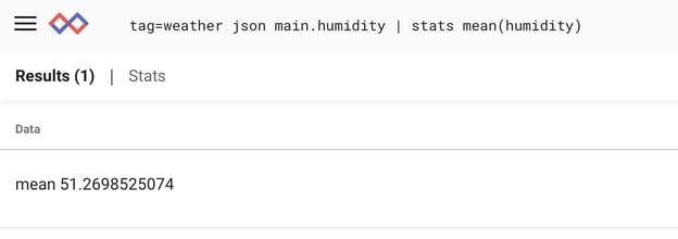
We can also see that the mean humidity in my city is a very comfortable 51%
So I have all the data I need, but how do I combine these datasets with compound queries? First, let’s break down the structure of compound queries.
What’s in a Compound Query
You can combine multiple queries together as a single "compound" query in order to leverage multiple data sources, fuse data into another query, and simplify complex queries. Gravwell's compound query syntax is a simple sequence of in-order queries, with additional notation to create temporary resources that can be referenced in queries later in the sequence.
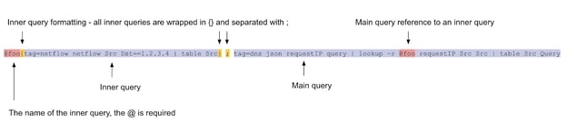
A compound query consists of a main query (the last query in a sequence), and one or more inner queries. You can have any number of inner queries, each with a unique name. Just remember that they execute one at a time and in the order you write them. The main query is written just like a normal query, while inner queries are always wrapped in the notation @<identifier>{<query>}. Queries are separated by a semicolon and whitespace doesn’t matter.
For example, below is a compound query that has 2 inner queries and a main query. Don’t worry about what the query is doing just yet.
@Q1{tag=default grep foo | json foo.bar foo.data};

@Q2{tag=syslog ax | table Event Payload};


tag=default ax
| lookup -r @Q1 match bar bar data
| lookup -r @Q2 Event Event Payload
Inner queries generate named resources in the form of @<identifier>. These can be used as regular resources with any module that supports table-based resources (such as lookup). Unlike real resources however, named resources in a compound query are ephemeral and scoped - they exist only while the query is running and are visible only to compound query in which they were created.
Let’s go back to our example from earlier and see if we can combine our weather data with our syslog events.
Example: Internet Stability and Weather - It’s Probably the Cloud...
We saw earlier that we have good historical humidity data as well as syslog notifications of service outages. Let’s use compound queries to simply annotate the current humidity at the time the syslog record arrived.
We’ll begin by building a table of the humidity at every minute (the granularity at which the weather kit gathers data):
tag=weather json main.humidity

| time -f “Mon Jan _2 15:04 2006 MST” TIMESTAMP tminute

| table tminute humidity
This gives us the humidity and a timestamp “tminute”, truncated to the minute.
We can make this query behave as a table-based resource simply by wrapping it in the compound query syntax. Let’s name this inner query “humidity”:
@humidity{

   tag=weather json main.humidity

   | time -f “Mon Jan _2 15:04 2006 MST” TIMESTAMP tminute

   | table tminute humidity

};
};
Finally, let’s reuse our query from above that extracts all network interruptions from syslog, and use the lookup module to enrich the entry with the current humidity:
tag=syslog ax value~”eth0: state INACTIVE”

| time -f “Mon Jan _2 15:04 2006 MST” TIMESTAMP tminute

| lookup -r @humidity tminute tminute humidity

| table value humidity
Finally, putting it all together, we get the following results:
@humidity{

   tag=weather json main.humidity

   | time -f “Mon Jan _2 15:04 2006 MST” TIMESTAMP tminute

   | table tminute humidity

};


tag=syslog ax value~”eth0: state INACTIVE”

| time -f “Mon Jan _2 15:04 2006 MST” TIMESTAMP tminute

| lookup -r @humidity tminute tminute humidity

| table value humidity
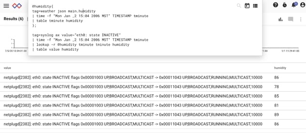
Well, look at that! The humidity is always high (compared to our mean of 51% we calculated earlier) when there’s a service outage.

Next, we’ll look at a more real world example.
Example: Enriching DNS and Connection Logs
For this example, we have both DNS query and IP-level connection data under the tags "dns" and "conns", and we want to filter connection data down to only connections that didn't first have a corresponding DNS query. We can use compound queries to enrich our first query with DNS data and filter.
Let's start with the inner query:
tag=dns json query answers | table query answers
This produces a table:
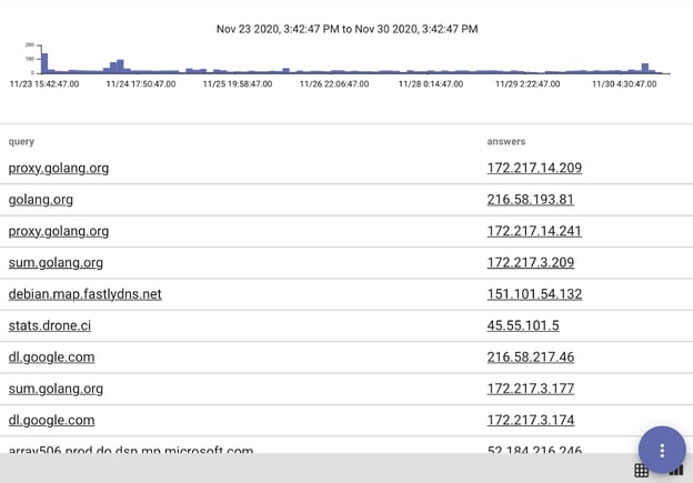
In the inner query, we simply create a table of all queries and answers in our DNS data. Since this is an inner query, we need to give it a name so later queries can reference its output, and wrap the query in braces. We'll call this inner query "dns":
@dns{tag=dns json query answers | table query answers}
In the main query, we use our connection data, and use the lookup module to read from our inner query "@dns":
tag=conns json SrcIP DstIP SrcIPBytes DstIPBytes
| lookup -s -v -r @dns SrcIP answers query

| table SrcIP DstIP SrcIPBytes DstIPBytes
This query uses the lookup module to drop (via the -s and -v flags) any entry in our conns data that has a SrcIP that matches a DNS answer. From there we simply create a table of our data.
We wrap this into a compound query simply by joining the queries together and separating them with a semicolon:
@dns{
tag=dns json query answers | table query answers
};
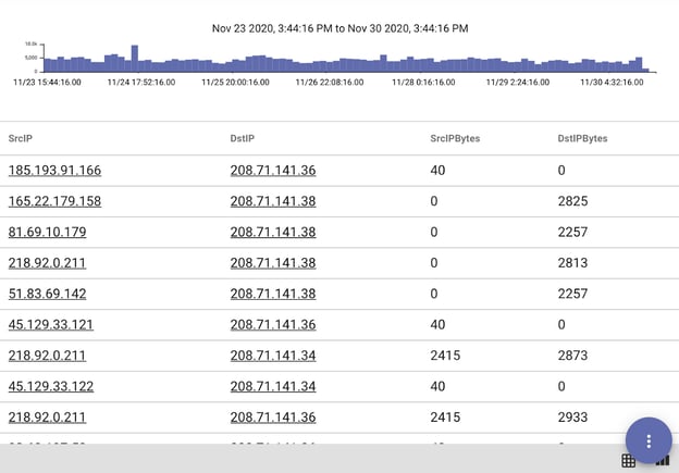
tag=conns json SrcIP DstIP SrcIPBytes DstIPBytes
| lookup -s -v -r @dns SrcIP answers query
| table SrcIP DstIP SrcIPBytes DstIPBytes
This gives us a table of just connections that didn't have a corresponding DNS query:
The Takeaway
Compound Queries are a powerful way to combine datasets in a single query, enabling data fusion and enrichment. Our support for compound queries will be expanding in future versions, so keep an eye out! To see compound queries and the other new features included in 4.1 in action, schedule a demo with one of our Gravwell Guides: